Put–call parity
In financial mathematics, put–call parity defines a relationship between the price of a European call option and European put option in a frictionless market —both with the identical strike price and expiry, and the underlying being a liquid asset. In the absence of liquidity, the existence of a forward contract suffices. Put–call parity requires minimal assumptions and thus does not require assumptions such as those of Black–Scholes or other commonly used financial models.
Contents |
Derivation
We will suppose that the put and call options are on traded stocks, but the underlying can be any other trade-able asset. The ability to buy and sell the underlying is crucial to the "no arbitrage" argument below.
First, note that under the assumption that there are no arbitrage opportunities, two portfolios that always have the same payoff at time T must have the same value at any prior time. To prove this suppose that, at some time t before T, one portfolio were cheaper than the other. Then one could purchase (go long) the cheaper portfolio and sell (go short) the more expensive. At time T, our overall portfolio would, for any value of the share price, have zero value (all the assets and liabilities have canceled out). The profit we made at time t is thus a riskless profit, but this violates our assumption of no arbitrage.
We will derive the put-call parity relation by creating two portfolios with the same payoffs and invoking the above principle.
Consider a call option and a put option with the same strike K for expiry at the same date T on some stock S, which pays no dividend. We assume the existence of a bond that pays 1 dollar at maturity time T. The bond price may be random (like the stock) but must equal 1 at maturity.
Let the price of S be S(t) at time t. Now assemble a portfolio by buying a call option C and selling a put option P of the same maturity T and strike K. The payoff for this portfolio is S(T) - K. Now assemble a second portfolio by buying one share and borrowing K bonds. Note the payoff of the latter portfolio is also S(T) - K at time T, since our share bought for S(t) will be worth S(T) and the borrowed bonds will be worth K.
By our preliminary observation that identical payoffs imply that both portfolios must have the same price at a general time  , the following relationship exists between the value of the various instruments:

where
 is the value of the call at time ,
 is the value of the put,
 is the value of the share,
 is the strike price, and
 value of a bond that matures at time
  . If a stock pays dividends, they should be included in , because option prices are typically not adjusted for ordinary dividends.
Note that the right-hand side of the equation is also the price of buying a forward contract on the stock with delivery price K. Thus one way to read the equation is that a portfolio that is long a call and short a put is the same as being long a forward. In particular, if the underlying is not tradeable but there exists forwards on it, we can replace the right-hand-side expression by the price of a forward.
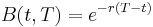
If the bond interest rate,  , is assumed to be constant then
-
Thus given no arbitrage opportunities, the above relationship (put-call parity) holds, and for any three prices of the call, put, bond and stock one can compute the implied price of the fourth.
Note: refers to the force of interest, which is approximately equal to the effective annual rate for small interest rates. However, one should take care with the approximation, especially with larger rates and larger time periods. To find exactly, use 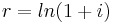 , where
  is the effective annual interest rate.
When valuing European options written on stocks with known dividends that will be paid out during the life of the option, the formula becomes:

where D(t) represents the total value of the dividends from one stock share to be paid out over the remaining life of the options, discounted to present value. This formula can be derived in similar manner to above, but with the modification that one portfolio consists of going long a call, going short a put, and D(T) bonds that each pay 1 dollar at maturity T (the bonds will be worth D(t) at time t); the other portfolio is the same as before - long one share of stock, short K bonds that each pay 1 dollar at T. The difference is that at time T, the stock is not only worth S(T) but has paid out D(T) in dividends.
We can rewrite the equation as:

and note that the right-hand side is the price of a forward contract on the stock with delivery price K, as before.
There is another way of thinking (and writing) the basic put-call relationship:

Both sides have payoff max(S(T), K) at time T, so this gives another way of proving put-call parity. The right-hand side is the value of a portfolio, a protective put, which is long a put and stock. The left-hand side is the value of a fiduciary call, which is long a call and enough bonds to buy a share of stock at time T if the call is exercised.
History
Forms of put-call parity appeared in practice as early as medieval ages, and was formally described by a number of authors in the early 20th century.
Michael Knoll, in The Ancient Roots of Modern Financial Innovation: The Early History of Regulatory Arbitrage, describes the important role that put-call parity played in developing the equity of redemption, the defining characteristic of a modern mortgage, in Medieval England.
In the 19th century, financier Russell Sage used put-call parity to create synthetic loans, which had higher interest rates than the usury laws of the time would have normally allowed.
Nelson, an option arbitrage trader in New York, published a book: "The A.B.C. of Options and Arbitrage" in 1904 that describes the put-call parity in detail. His book was re-discovered by Espen Gaarder Haug in the early 2000s and many references from Nelson's book are given in Haug's book "Derivatives Models on Models".
Henry Deutsch describes the put-call parity in 1910 in his book "Arbitrage in Bullion, Coins, Bills, Stocks, Shares and Options, 2nd Edition". London: Engham Wilson but in less detail than Nelson (1904).
Mathematics professor Vinzenz Bronzin also derives the put-call parity in 1908 and uses it as part of his arbitrage argument to develop a series of mathematical option models under a series of different distributions. The work of professor Bronzin was just recently rediscovered by professor Wolfgang Hafner and professor Heinz Zimmermann. The original work of Bronzin is a book written in German and is now translated and published in English in an edited work by Hafner and Zimmermann ("Vinzenz Bronzin's option pricing models", Springer Verlag).
Its first description in the modern academic literature appears to be (Stoll 1969).[1]
Implications
Put–call parity implies:
- Equivalence of calls and puts: Parity implies that a call and a put can be used interchangeably in any delta-neutral portfolio. If
 is the call's delta, then buying a call, and selling shares of stock, is the same as buying a put and buying
  shares of stock. Equivalence of calls and puts is very important when trading options.
- Parity of implied volatility: In the absence of dividends or other costs of carry (such as when a stock is difficult to borrow or sell short), the implied volatility of calls and puts must be identical.[2]
References
- ^ Cited for instance in "The illusions of dynamic replication", Emanuel Derman and Nassim Nicholas Taleb, 2005
- ^ Hull, John C. (2002). Options, Futures and Other Derivatives (5th ed.). Prentice Hall. pp. 330–331. ISBN 0-13-009056-5.
- Stoll, Hans R. (1969). "The Relationship Between Put and Call Option Prices". The Journal of Finance 24 (5): 801–824. doi:10.2307/2325677.
External links
- Put-Call parity
- Put-Call Parity and Arbitrage Opportunity, investopedia.com
- The Ancient Roots of Modern Financial Innovation: The Early History of Regulatory Arbitrage, Michael Knoll's history of Put-Call Parity
- Other arbitrage relationships
- Arbitrage Relationships for Options, Prof. Thayer Watkins
- Rational Rules and Boundary Conditions for Option Pricing (PDFDi), Prof. Don M. Chance
- No-Arbitrage Bounds on Options, Prof. Robert Novy-Marx
- Tools
- Option Arbitrage Relations, Prof. Campbell R. Harvey
|
|||||||||||||||||||||||||||||||||||||